class: center, middle, inverse, title-slide # Session 5 --- ## The pipe operator - It can be written as %>% or |> - Makes your code more clear ```r mutate(x, y=x+1) # same as x %>% mutate(y=x+1) # or x |> mutate(y=x+1) ``` - Use a keyboard shortcut to put it in a script! - In my mac is Ctrl+Shift m --- # Why? - With the pipe operator we can chain multiple functions together. - Calculate mean total points grouped by playoffs. .pull-left[ ```r nba <- readRDS('./nba.rds') nba_grouped <- group_by(nba, Playoff) nba_summary <- summarize(nba_grouped, avg_pts=mean(PTS)) ``` ] .pull-right[ ```r nba_summary <- readRDS('./nba.rds') %>% group_by(Playoff) %>% summarize(avg_pts=mean(PTS)) ``` ] --- ## Rmarkdown - File format for reports. - It combines R code and text. - It generates documents (pdf, word, html). 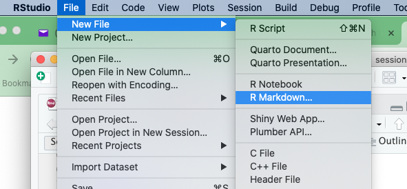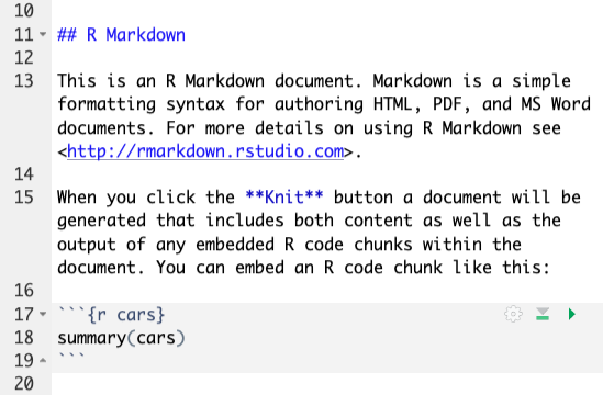--- ## Create a file inside your project  --- ## Contents  - Line 11 is text (level 2 header). - Line 15 is regular text. - Lines 17-19 are R code --- ## Rmarkdown - R __code chunks__ appear between 3 backticks (`). - When we run the file, R runs all the code inside this chunks and puts the output in the final document. - Ctrl+Shift+i inserts a code chunk. 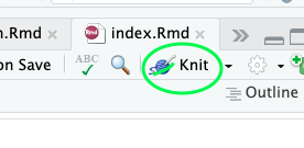- Outside the tags, your can use _markdown_ --- ## Knit - Press the knit button to generate the final document (pdf, word or html file).